Test a meta-reinforcement learning model (A2C) on an associative learning task.
Test a meta-reinforcement learning model (A2C) on an associative learning task
In this post, I want to explore the power of a simple meta-reinforcement learning (meta-RL) model on simple associative learning tasks. This is the second post on my journey to understand meta-RL models and hopefully tweak them to behave like humans; and you can check out my overall project proposal here. This post assumes that you have basic knowledge on reinforcement learning (RL), and there are plenty of good RL tutorials out there.
What is meta-reinforcement learning?
The term “meta” confused me for a long time, so let’s understand “meta-learning” in a clearer term: learning to learn. Imagine the traditional way we train a RL model to play the Pong game. For example, we can decide to pick the DQN algorithm, specify the number of layers and units in the Q-network, and finally choose our favorite loss function and optimizer. We may get lucky this time and the model plays Pong well, but this combination of choices may not work for the GO game, and we need to start from scratch and test numerous other algorithms. What if we can train a model to learn the best learning algorithm for the task? Wouldn’t it be wonderful if we have such a model that can figure out the best way to learn in the current task setting? This is the essence of meta-RL models: find the best learning aglorithm for the task with reinforcement learning.
Why should we test the model on associative learning tasks?
Associative learning tasks are pretty common in the cognitive science field but not so much in computer science, but in our context they are simple multi-armed bandit tasks. You might think that multi-armed bandit task is one of the most basic problems in RL and countless algorithms are already built to solve it near-optimally, why bother testing it? Well, here are several reasons:
-
Most of RL algorithms have built-in memory one way or another, but meta-RL algorithms don’t. Traditional models keep information of rewarding state-action pairs in Q-tables or value networks, so the way they utilize these memory resources are designed by the human researchers. On the other hand, the learning algorithms learned by meta-RL models are complete black boxes; researchers only specifies the number of memory units that the learning algorithm can use, and how these memory units are used is totally up to the algorithm. **By testing the meta-RL algorithm on associative learning tasks, we hope to understand how they utilize the given memory resources.
-
While researchers can easily expand the memory resources in RL algorithms, you can’t do the same things to humans. Humans have very limited memory resources, and their performance fell short even in simple associative learning tasks as the number of state-action pairs increases. However, humans seem to recognize this limit and they can act in a near-optimal fashion under this constraint. It is therefore intriguing to see whether the learning algorithm learned by the meta-RL model can show similar behavior under limited memory resources.
Let’s quickly go through the procedure of the associative learning task. As shown in Fig. 1, the model was trained on multiple associative learning blocks which have either 3 or 6 objects. At the start of each block, each object will be randomly associated with one of the three buttons. For each trial within each block, the model observes one stimulus (one-hot encoded in the experiment), presses one of the three action buttons, and finally gets feedback on whether the object-action pair is correct or not. I tried to replicate this procedure described in this paper as they recruited human participants to do this exact same task, and this makes it possible to compare the behavior between humans and models.
The associative learning task
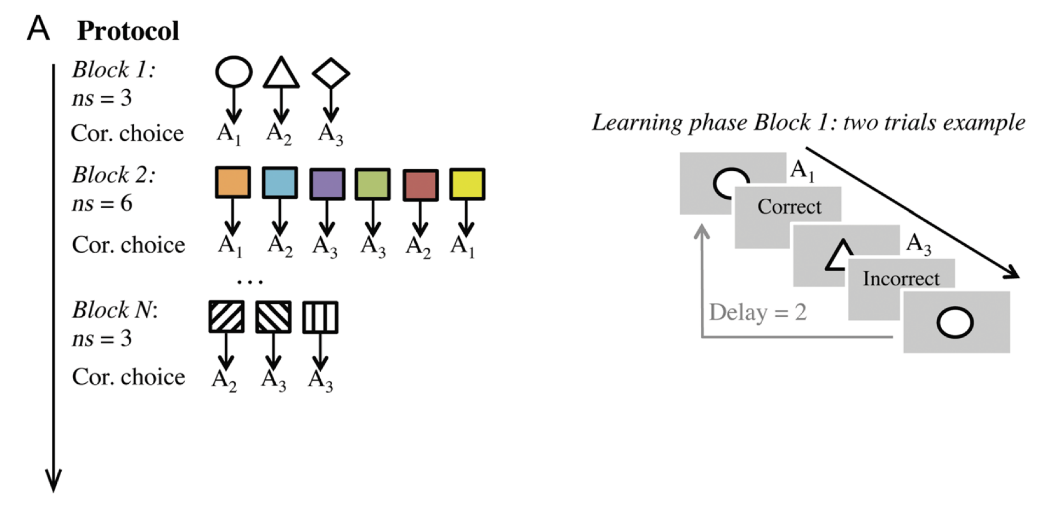 Fig. 1. Experiment procedure of the associative learning task. Figure adapted from [1]
Now it’s time to train some models!
First, let’s setup the environment
import numpy as np
import pandas as pd
import matplotlib.pyplot as plt
import matplotlib as mpl
%matplotlib inline

plt.style.use('seaborn-dark-palette')
mpl.rcParams['axes.titlesize'] = 20
Second, let’s train the model
I trained an iconic meta-RL model, an A2C algorithm with 50 LSTM units, on 40 million trials. I compared the behavior between human participants and the trained meta-RL model.
To examine how meta-RL models behave under limited memory resources, I trained another model with 20 LSTM units on 20M trials. Reducing the number of LSTM units is definitely a crude way to limit memory resources, but it does the work as a first step. I will explore various capacity-limited model variants (e.g. limit the mutual information between observation and action) in the future.
from envs.Collins2018 import Collins2018Task
from utils.utils import do_experiment

# specify the agent and the environment
num_lstm_units = 20
num_train_steps = 20_000_000
policy_kwargs = {'n_lstm': num_lstm_units, 'action_noise': 0}
env = Collins2018Task(num_objects=(3, 6), num_actions=3, num_repeats=13)

do_experiment(env, num_train_steps, policy_kwargs)
Finally, let’s use the learned model to rollouts some new blocks.
To test whether the learned model can generalize to new tasks, we rollout the model on 600 new blocks where 1 to 6 objects are available. Note that this isn’t really testing whether the model can transfer knowledge from training tasks to new tasks: The model can probably solve 1 to 5-object blocks just like 6-object blocks where the remaining object are absent. It is still good to test whether the model can reach this level of generalization though.
You might encounter tons of warnings if you are running this notebook. This is because I am using the A2C implementation from stable-baselines which uses tensorflow v1.
from utils.utils import Simulation
from envs.GuessBoundary import GuessBoundaryTask
from envs.Collins2018 import Collins2018Task

env = Collins2018Task(num_objects=(1, 2, 3, 4, 5, 6))

sims = [
    Simulation('./outputs/Collins2018/A2C-LSTM50', env, load_params_file_idx=20_000_000),
    Simulation('./outputs/Collins2018/A2C-LSTM50', env, load_params_file_idx=10_000_000),
    Simulation('./outputs/Collins2018/A2C-LSTM20', env, load_params_file_idx=20_000_000)
]

for sim in sims:
    sim.evaluate(num_test_episodes=600, num_trials=100, verbose=True)
Let’s check the model’s training progress
from utils.visualization import plot_training_progress

plot_training_progress(sims[0].model_path)
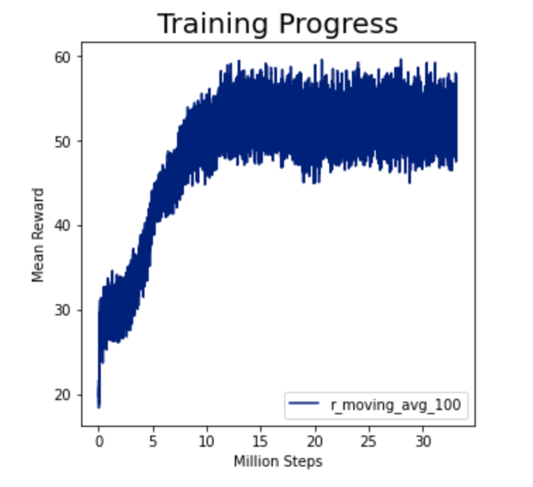
The model with 50 LSTM units probably reached performance plateau after 15 million trials of training.
Let’s compare three models:
- a 50-unit A2C model trained with 20M trials (possibly over-trained)
- a 50-unit A2C model trained with 10M trials (possibly under-trained)
- a 20-unit A2C model trained with 20M trials (possibly over-trained)
Let’s compare how human participants score against the meta-RL model
from utils.visualization import plot_associative_learning_progress, calc_exploration_and_retention
from utils.utils import behav2sim

df_behav = behav2sim()
dfs = [
    df_behav,
    sims[0].rollouts,
    sims[1].rollouts,
    sims[2].rollouts
]
mdl_names = [
    'human behavior',
    'LSTM50 / train20M',
    'LSTM50 / train10M',
    'LSTM20 / train20M'
]

fig, axs = plt.subplots(1, len(dfs), figsize=(16, 4))

for mdl in range(len(dfs)):
    # does the model learn after multiple stimulus presentations?
    plot_associative_learning_progress(axs[mdl], dfs[mdl])
    axs[mdl].set_title(mdl_names[mdl])
    # does the model learn to attempt different actions after failed trials (before the single success)?
    #calc_exploration_and_retention([axs[1, mdl], axs[2, mdl]], dfs[mdl])


# insight: network should be quite larger than the optimal size
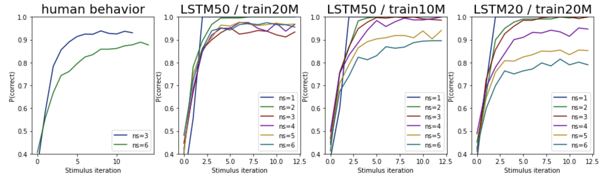
You can see how the human participants score against the three models.
The main highlight here is that human participants did worse in the 6-object blocks than the 3-object blocks (leftmost figure). This is expected since humans typically can’t remember this many object-action pairs, so they need a bit of extra practice to reach the same level of performance. The over-trained model (second figure) doesn’t show this obvious trend, but the under-trained and memory-limited model shows similar trend.
Now let’s do a more detailed analysis on how the models utilize memory.
To examine that, we can check the following two aspects:
- If the make a wrong action guess, it should try another action during the next encounter. Since there is only 3 action buttons, for each object the maximum number of failed attempts before the correct action is hit is at most 2. More than 3 failed attempts shows imperfect memory on the incorrect action attempts.
- After the correct action is selected, the model should stick to this action for the rest of the block. Failure to do so shows imperfect memory on the correct action attempts.
fig, axs = plt.subplots(2, len(dfs), figsize=(16, 8))
axs[0, 0].set_title('human behavior')
axs[0, 1].set_title('LSTM50 / train20M')
axs[0, 2].set_title('LSTM50 / train10M')
axs[0, 3].set_title('LSTM20 / train20M')

for mdl in range(len(dfs)):
    # does the model learn to attempt different actions after failed trials (before the single success)?
    calc_exploration_and_retention([axs[0, mdl], axs[1, mdl]], dfs[mdl])
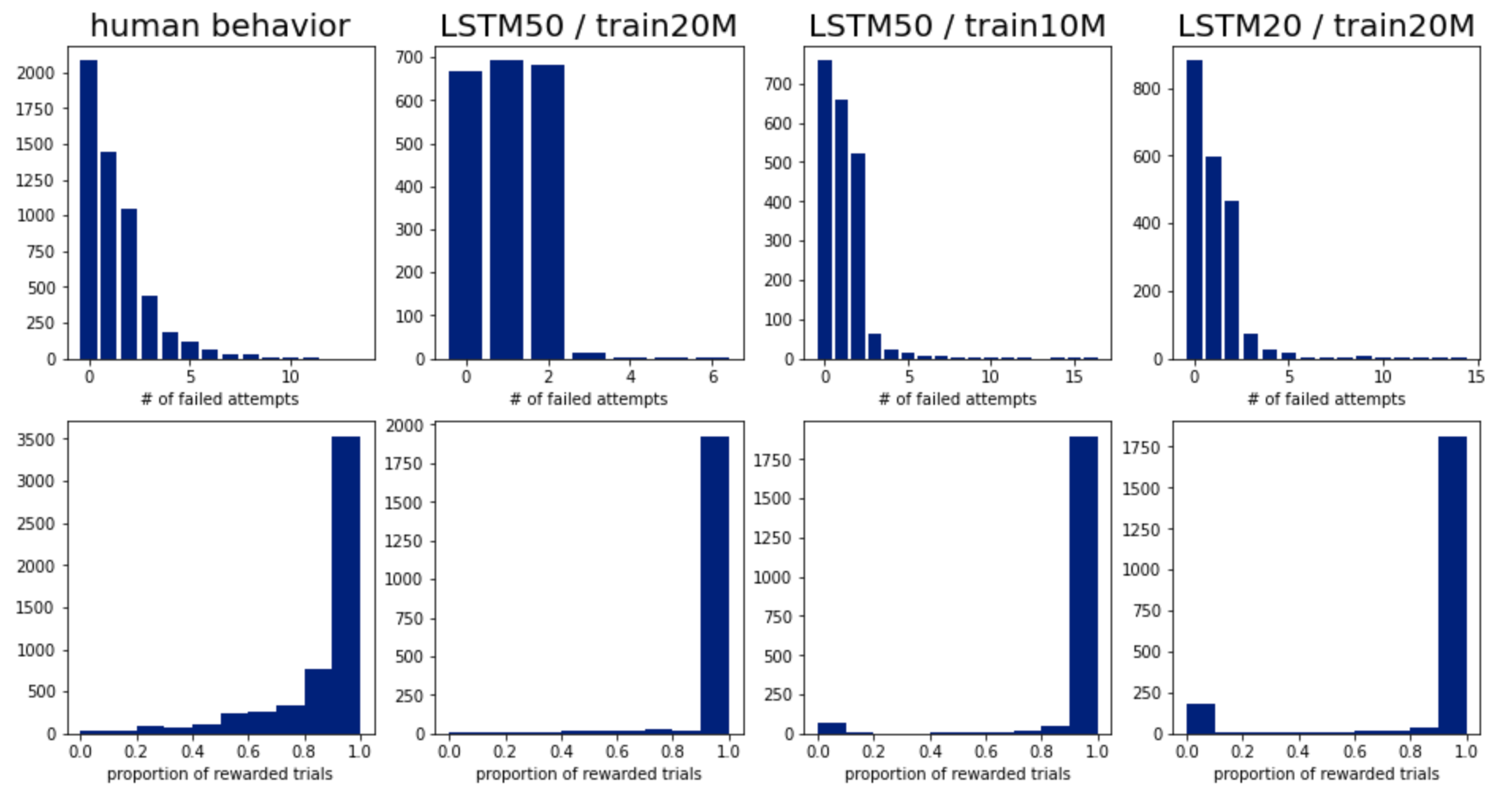
The top row shows the distribution of number of failed attempts before the correct action is found. We can easily observe that humans occasionally forget the incorrect actions they have picked in the previous trials. The models, especially the over-trained one, show almost perfect memory on previous incorrect attempts.
The bottom row shows the distribution of average reward after the correct action is found. All the points should be at 1.0 if the model can remember the correct action perfectly. We can see that the over-trained model is nearly perfect, and humans again show some level of imperfect memory.
Note the small bump at 0 in the bottom right graph. What does this mean? This means that the trained model has a noticeable chance to completely forget the answer for an object. This shows that the model fails to consistently utilize its memory resources. More training can certainly solve the problem, but this might mean the models are using memory in a fundamentally different way as humans do.
Are there more artifacts unique to the models?
You bet. Since the objects are coded 0-2 and 0-5 in the 3- and 6-object tasks respectively, the model may be trained more on the first three objects and less the last three. On the other hand, humans subjects might show similar trends since their working memory is already pre-occupied by earlier objects, but the effect shouldn’t but huge.
Here is the comparison between the human behavior and the model:
# is there training artifact that the stimulus 0-2 are better trained?
# Ans: yes
fig, axs = plt.subplots(1, len(dfs), figsize=(16, 6))

for mdl in range(len(dfs)):
    obj_rewards = dfs[mdl].groupby('observations').rewards.mean().tolist()
    axs[mdl].bar(np.arange(len(obj_rewards)), obj_rewards)
    axs[mdl].set_title(mdl_names[mdl])
    axs[mdl].set_xlabel('Object ID')
    axs[mdl].set_ylabel('Mean Reward')
    axs[mdl].set_ylim([0.5, 1])
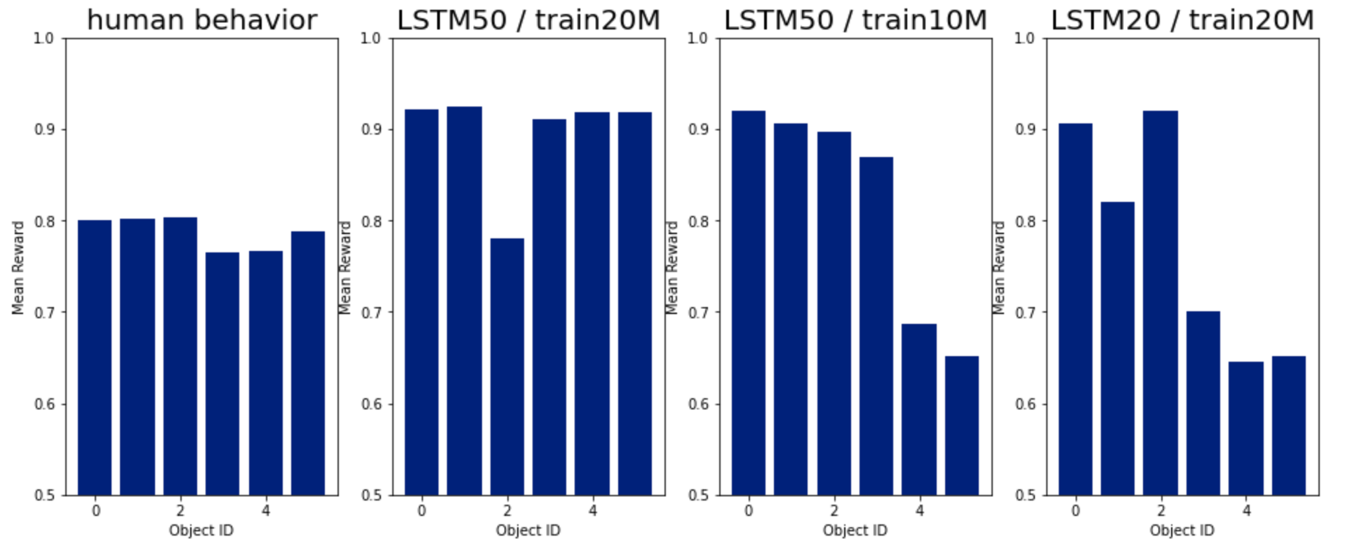
Hmm, that is messy. As expected, humans are pretty consistent across different objects; as long as a red circle looks different from a green one, we should have no trouble associating them with different actions. For the under-trained and the memory-limited models we can see a drop for the last three objects, probably because they received 50% less training. The third object in the over-trained model oddly shows lower performance, and I haven’t figured out why yet.
Nevertheless, one thing is for sure: while humans can easily identify that the same rule can be applied to all objects regardless of how many they are, models probably learn the rule of each object independently. This partially explains why it takes 20 million trials to train a meta-RL model to learn such a simple associative learning task. This is one of the advantages of graph neural networks (GNNs) over plain LSTM units: if the memory resources given to a meta-RL model is a graph instead of a fixed-sized network, the model may opt to create a memory node for each object it encounters and learn a single operation that applies to all nodes. The latter usage of memory is much closer to humans and it needs way fewer parameters. In the next post, I will explore how such networks can be implemented and how they behave on this associative learning task.
Conclusion
In this post, I examined how a meta-RL model utilizes its memory resources and compared it to human behavior. I trained multiple models on a simple associative learning task and found that while models often memorize important information better than humans do, they require a huge amount of training data and they tend to learn the rule for each object independently. In the future posts, I will explore how to enforce stronger inductive biases into a meta-RL model and force it to learn in a human-like manner.
This is only a work in progress and there are still quite a lot of TODOs to clean up:
-
While behaviors can tell us a lot about how models utilize memory, it is even better if we can directly infer what is stored inside the LSTM hidden units. One way to do this is to correlate task-relevant information (e.g. which objects are already associated with action buttons) through multiple blocks with the hidden state values. This yields mixed results in my previous attempts, but I think this might be worth a shot.
-
Limiting the memory resources of a model by reducing the number of LSTM units is definitely a crude approach, and there are more elegant information-theoretic approaches that I have yet explored. A meta-RL model can be interpreted as a capacity-limited channel that maps observations to actions, and this capacity can be tuned by limited the mutual information between the model input and output. It will be interesting to see whether enforcing such mutual information constraints can make the meta-RL model behave more like humans.
References:
1.Collins AGE. The Tortoise and the Hare: Interactions between Reinforcement Learning and Working Memory. J Cogn Neurosci. 2018 Oct;30(10):1422-1432. doi: 10.1162/jocn_a_01238. Epub 2018 Jan 18. PMID: 29346018.